
In my youth, I fostered an interest in the electrical signals generated by the body and more recently in how the body reacts to them. I am now quite interested in Neuroscience and am working to promote the reading and induction of electrical signals into the human body without having to touch the body or use implanted technologies.
I am not a funded researcher and am not biased towards any software or hardware provider – I am doing this out of my own personal interest. I hope this tutorial to help those starting out. In this tutorial I outline which technology I purchased, the reasons for, and present a walk-through to help those new to this technology quickly come up to speed. Note that the software referenced below is now dated, there is newer software available.
Which hardware to buy?
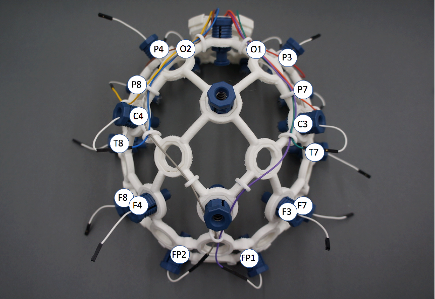
If I used hardware that conformed to industry standard, then my results would be comparable with others, so I chose to use the 10/20 Position reference system as it covers the areas often monitored by scientists conducting studies, and has the least number of electrodes (reducing costs).
My criteria:
- I want as close to research grade quality EEG recordings as possible.
- It must conform with the 10/20 position standard, as this will help to ensure the unit conforms to an electrode placement standard.
- I did not want to have to use gel based electrodes as they take a long time to apply.
- It must be affordable.
I reviewed the following products: Emotive, Neurosky, Versus, Muse, OpenEEG, and OpenBCI. I did not pursue the OpenEEG unit even though it offers a higher electrode count, because I did not feel comfortable in building it myself as I felt that any recorded signals could then be subject to scrutiny as there is no guarantee that I had built the device correctly or that all of the components were within spec. So I chose the OpenBCI solution as it offered the best EEG coverage (highest electrode count, full range EEG recording, and 24 bit sampling) – and was within my price range. I purchased a Cyton and Daisy Biosensing board, the UltraCortex “Mark IV” headset, and a set of Florida Research Instruments 5mm Spike disposable dry EEG electrodes. The Cyton and Daisy Bio-sensing board allow me to record 16 channels (16 inputs) of EEG, EKG, or a mixture of both. The UltraCortex headset allows consistent placements of the electrodes on my head, with the electrodes being height adjustable and easy to put on. The 5mm Spike disposable dry EEG electrodes work well with medium length hair, are comfortable, but have a short life span. However, the electrodes are very easy to replace, with one Phillips screw holding them in, and are cost effective.
Hardware setup issues
When I first started to use the unit, I discovered that the OpenBCI on-line guide was inaccurate as to the wiring of the UltraCortex Mark IV Headset, causing my Cyton to “Rail” on all signals. Railing is when a signal cannot be properly interpreted, so it is ignored. I reviewed the OpenBCI Forums and figured out the correct way to wire the headset, and provided my findings to OpenBCI so that they could update their tutorial. I encourage you to follow their updated instructions, but perhaps make sure that:
- the left ear wire is connected to the BIAS pin on the Cyton that is closest to the board
- the right ear wire is connected to the SRB pin on the Cyton that is closest to the board
- you use the provided white splitter cable to connect the SRB pin closest to the board on the Cyton with the SRB pin closest to the board on the Daisyboard as this keeps the reference signal the same between the two cards
- notice that the BIAS pins are not connected to anything on the Daisyboard.
Regarding the above described pin connections, note that the Cyton is installed in the headset, and that I am holding the headset upside down.
After correcting the wiring the unit worked flawlessly, railing only when you needed to change an electrode or when an electrode was not properly seated on the skull (light pressure should be felt). Note that electrodes need to be replaced when the conductive coating starts to come off the electrode tips.
Further confusion! Two 10/20 position standards!
And just to add to the fun I later noticed that there are two 10/20 standards! The newest is the International 10/20 EEG placement system. The OpenBCI tutorial now correctly identifies the EEG electrodes as according to this newest standard. But in case you find references to older documentation, note that T3, T4, T5, and T6 were updated to be T7, T8, P7, and P8 respectively!
My first attempts…
I recorded EEG using the provided Bluetooth dongle and software. I wanted to analyze the recorded signals, so I downloaded a stand-alone version of EEGLAB. There is a lot of information about this software on the EEGLAB website. EEGLAB uses the free MATLAB executable, so I was able to import my signals, apply filters, remove noise, and view my EEG readings at no cost!
But I ran into two problems using this technology initially……
The first was that EEGLAB was written to be used by researchers, and had way more features and requirements than I needed as a home researcher – forcing me to take a long time to set up and run experiments. I wanted to learn how to review EEG signals myself, so I purchased the “Home Use” version of MATLAB and used it. I downloaded the EEGLAB plug-in (which is kept more up to date), just in case I wanted to use it in the future!
The second problem was with the Cyton and Daisyboard. While working with EEGLAB I discovered that I had not quite understood how the Cyton worked when you sample using Bluetooth. I was not sampling at 250Hz as I had thought – I was actually only sampling at 125Hz because the Cyton generates more data than Bluetooth bandwidth can handle! In this mode the Cyton “Averages” the signal data by taking an average of the current and most recent channel values before sending them. This means that the very first sample sent is not valid as there is no previous sample to average it against – therefore it must be removed prior to analysis. While using Bluetooth is convenient because the data is recorded directly on your PC, it does not provide you with the highest possible data quality. To fix this, I started to use the Cyton’s built-in Micro-SD slot as it can be used to record all 16 EEG channels at the full 250Hz sampling rate. In this method, the raw (un-averaged) data is written directly to the SD-Card. Because of the high data transfer speeds required to record all of the signal data to the SD Card, a special file format is used for the recorded file. This file format creates a space on the SD Disk that the data will be written into, this means that after the data is recorded you must copy the file to your computer and then use the provided software to convert it into a more usable format. To me, this is a small price to pay to get high-quality EEG recordings!
It might be interesting for you to know that the Cyton will record 8 signals during one sampling and the second 8 from the Daisyboard during the next sampling (Cyton values for odd samples and Daisyboard values on even samples).
Tutorial Start
I will now outline to you the steps I followed to install the older version of the OpenBCI software on your computer, use it to record EEG signals onto the SD-Card, copy the EEG data file to the computer, and then review the information in MATLAB Home Edition.
Step 1) – install the software
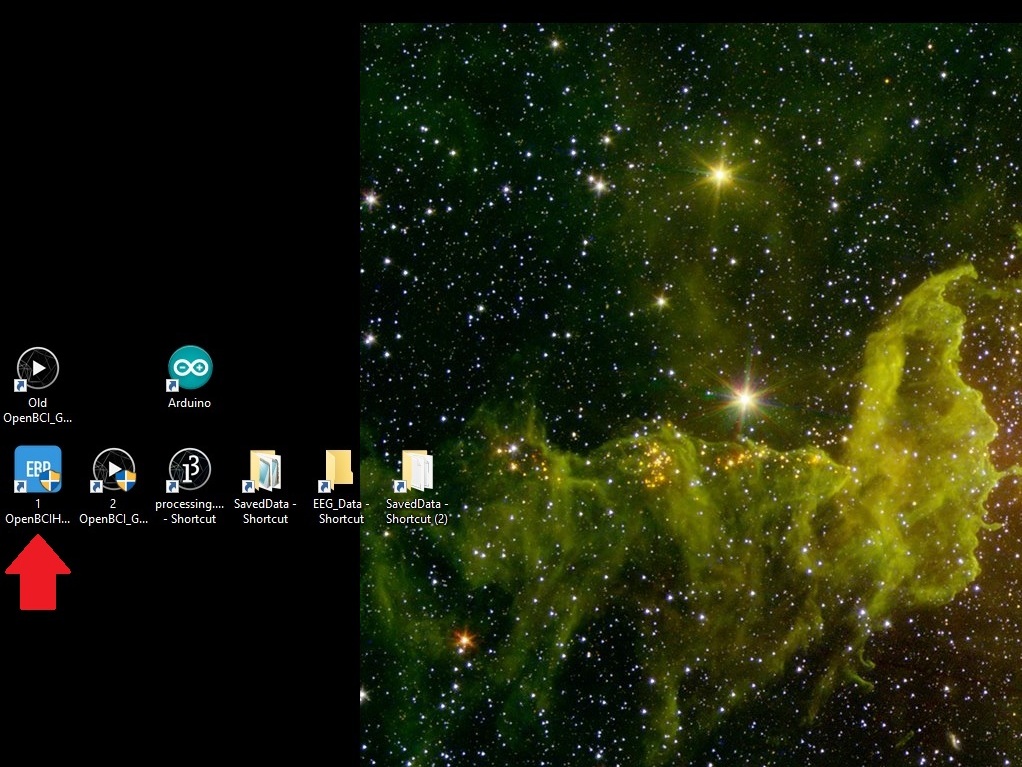
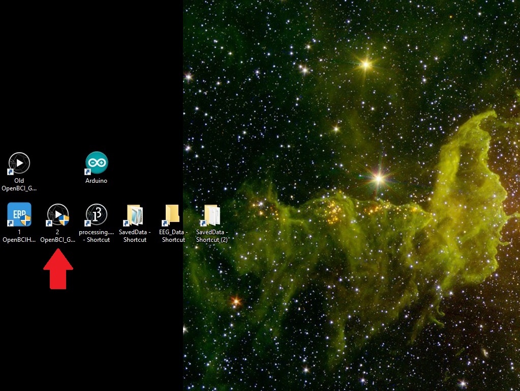
The latest version of the OpenBCI software uses a Windows Service to communicate between the hardware and software devices necessary for the software to work. Install the OpenBCI Recording and Visualization software on your computer by following this tutorial. To help make it easier to use the software, I made shortcuts to the applications onto my Windows Desktop, and then numbered them as pictured below (programs 1 and 2).
Step 2) – prepare a script
When you are ready to analyze your EEG data in MATLAB you will need to remember what you did while you were making the recording. I always create and follow a timed ‘script’. This allows me to view my EEG data and locate the artifact responsible for the action (ex. blinking an eye every 10 seconds). As different parts of the brain are responsible for different actions performed by the body, this link will help you identify which part of the brain would be generating the artifact you are looking for – and you can then figure out which electrode would have captured the signals. Once you figure out what you want to do, create a timed script that you will follow.
Step 3) – how to run the software
You must double-click on the OpenBCI Hub program first (I labelled it program 1). When prompted, choose to allow the software to make changes to the computer.
Step 4) – how to open the interface
Now that the service is running, double click on the OpenBCI GUI shortcut (program 2). When prompted, choose to allow the software to make changes to the computer.
Step 5) – record the signals
In the video below, I show how to use the OpenBCI GUI to record signals directly to the SD Card on Cyton. As I have a Daisyboard, I choose to record 16 EEG channels. I selected to record a 5 minute long file. Note that once the application opens, I choose “Auto” for the Vertical Scale, for best viewing of the EEG signals. I also change to display the Head Plot, so you can see which areas are the most active. I click “Start Data Stream” to start recording. When the signals are first being recorded, there is a large spike generated across all of the EEG channels – this is normal and will need to be removed during signal analysis. After a couple of minutes I click “Stop Data Stream” to end the recording. I then click “System Control” and “Stop System” to tell the Cyton to stop recording and to create the file on the SD card.
Step 6) – download the file to the computer
Physically remove the SD Card from the Cyton, put it into the USB Key provided with the unit, and then plug the USB Key into the computer. If it is a recording I’d like to keep, I put a copy in my archives – renaming the file to a more meaningful name. Reference the video below to see how I use the OpenBCI GUI to convert the file.
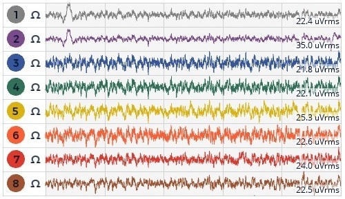
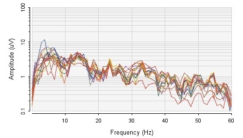
I had many requests to provide my EEG so that people could follow along with my demo – so I recorded 4 minutes of EEG for this example, and offer the raw SD Card file and the converted file here (file called EEG.zip). If you review my signals you’ll note spikes – this is not noise or malfunctioning equipment – I was clenching my jaw, moving parts of my body, and performing a number of rapid eye blinks. Muscle movements can be easily detected by reviewing frequencies 40Hz and above.
Congratulations – if you’ve made it this far then you have successfully made your first recording! Now let’s review them!
Using MATLAB to clean up the recordings
I had never used MATLAB prior to this so I struggled with how to code with it and prepare the data files for analysis. My hope is that this section will help those also new to this, and that you will be able to re-use my code for your own purposes. As per my setup, this code is written to work with a 16 Channel data set that was recorded onto the SD-Card (which ends up using the OpenBCI format which is a Comma Separated File). Because we are recording EEG data to the SD-Card on the Cyton, the sampling frequency is 250Hz – therefore we have to use Nyquist Theory to determine the highest frequency we can sample. This calculates to: 250Hz / 2 = 125Hz. As well, in this example I am not concerned with frequencies less than 3Hz.
In general, the function of all this code is to: import and condition the samples, apply filters, and generate sample numbers so that they can be aligned against the prior mentioned timing script (step 2). I’ve broken my code into segments to help identify what each section does. I recommend that you review the code prior to running as I often put variables at the top that must be set properly for the code to run (file names, etc.). Using comments, I’ve broken this MATLAB code into the following segments:
- Import Raw Data
- the EEG data is comma separated – some lines have gyroscope and acceleration data
- you must remove the top three lines of the data (header)
- you must remove the last few lines (14) from the data (some sort of logging data)
- a temporary CSV file is created to store the data slice
- import the data from that temporary CSV file into a MATLAB variable
- temporary variables and files are removed
- Remove the accelerometer and gyroscope data
- the data is in columns – I remove the gyroscope and acceleration columns as I do not have a use for them
- Copy the data into a new variable
- the data is transposed into rows so it can be more easily used in MATLAB
- Separate the data into separate channels (variables)
- name each channel appropriately
- Apply a zero phase digital high pass filter
- 5Hz and above with a 3Hz stop
- Apply a zero phase digital 60Hz notch filter
- removes any 60Hz interference from hydro sources
- Apply a zero phase digital low pass filter
- 122Hz and below with a 125Hz stop
- Use the Timer_Raw data to number each of the samples and show time lapse between samples
- helps when plotting graphs and to find and identify epochs
- Clear temporary variables
The MATLAB plot below shows the differences between the signals prior to, and after applying the signal conditioning.
NOTE: For those who wish to use the Bluetooth method, I offer the following code below. This Bluetooth code is different as it considers that the file structure is different from the method used when saving to the SD Card. When using Bluetooth, the unit can only send 8 of the 16 channels data during each sampling – so the unit alternates the writing of data. In other words, on the first sampling the first set of 8 channels of data is written to the file, then on the second sampling the second set of 8 channels is written to the file. This continues until the session is complete. Remember that even though the Cyton is set to sample at 250Hz it will only sample at 125Hz due to the Bluetooth speed restriction, therefore all of the filters and such have been modified to remove the appropriate frequencies and condition the signals. Use this code HERE to decode signals generated by Bluetooth.
Reviewing and cleaning the Signals
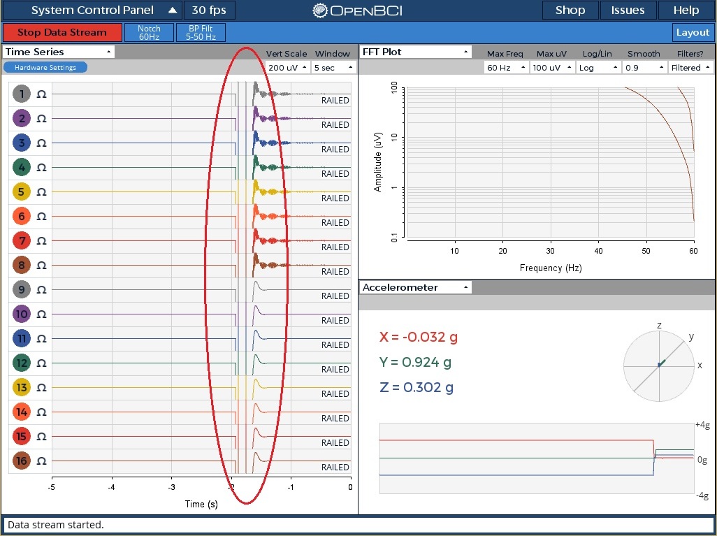
Prior to using and referencing the signals, we have to ensure their quality. The Cyton will initialize the channels when you start recording. To help visualize this, I took a screen shot of the OpenBCI software after having started recording. I circled the signal initialization segment in the image below. Note that each channel is railing in the picture as I was not wearing the headset.
Prior MATLAB filtering applied to the data may have eliminated some of this signal settling, but will not have removed all of it. In fact, you may have a ‘blank’ section at the beginning or end of your signals. You can run the following MATLAB command below at the MATLAB prompt to review the signals and see how much of the signals need to be removed. (MATLAB Code – see Step 1 in code)
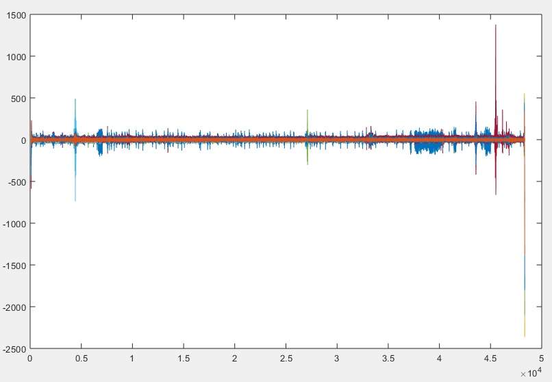
You will then want to review the beginning and end of the data stream, to ensure that there are no blank (zeroed) sections. If you are familiar with the plot tool, you can use the zoom tool to review the beginning and end of the signal. Or, we can check this by running the following MATLAB code (link below) which allows us to zoom into the first 400 samples in step 2. In this example, I will plot C3_Filtered data throughout. (MATLAB Code – see Step 2 in code)
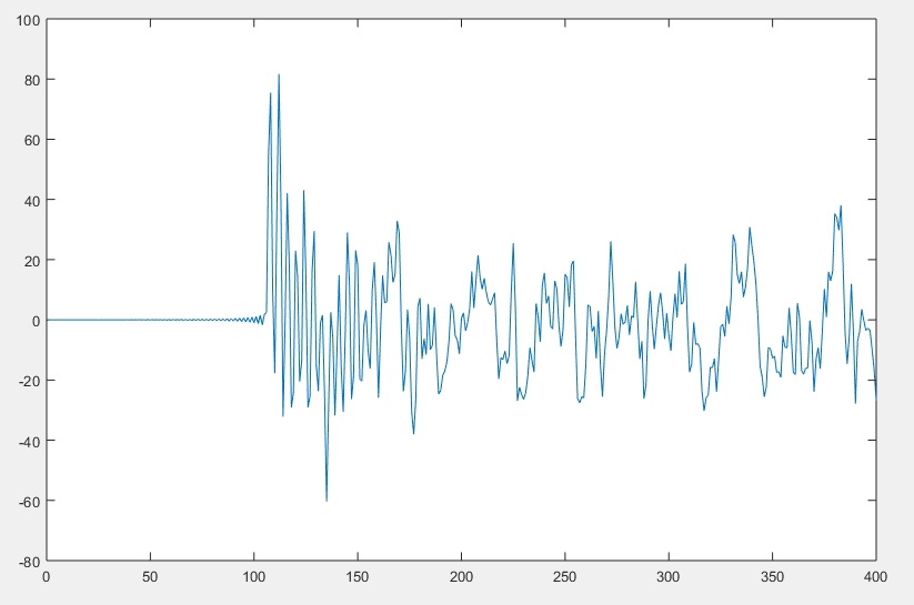
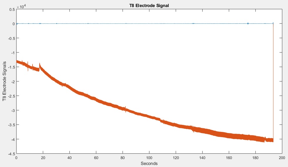
As can be seen in the image above, the first 106 samples do not contain any signals having any value. Therefore we will have to remove the first 106 samples (approximately 0.5 seconds of data) from all of the signals. Of course, the code will also adjust the sample count and sample timer – otherwise your recorded signals would no longer be in sync with your script. Note that I used the variable X in the code, to easily allow you to adjust it to any length. After running the MATLAB code, I reviewed the C3 data (below). (MATLAB Code)
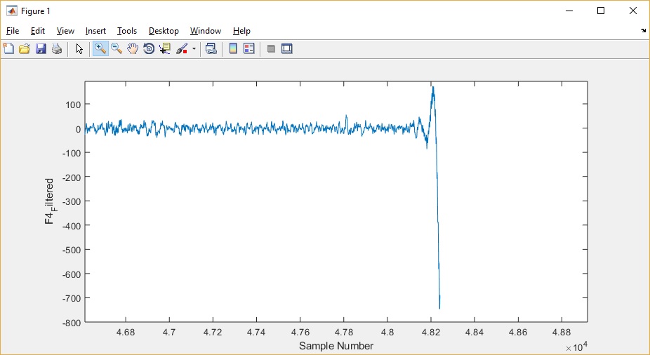
I plotted other signals, and in plotting F4_Filtered noticed that there was an anomaly at the end of the signal. I used the Zoom tool (circled below) to zoom into the signal to see how many samples I needed to remove.
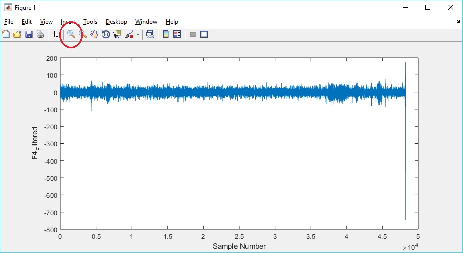
In reviewing the zoomed in signal, I decided to remove the last 60 samples. I remodeled the code to accommodate removing from the end of all of the signals (to keep all of the signals in sync).
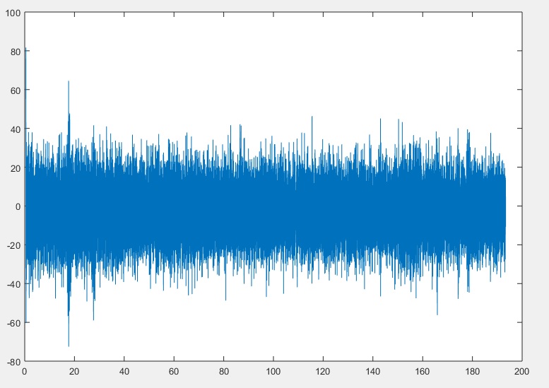
After running the MATLAB code, I plot F4_Filtered again (below). (MATLAB Code)
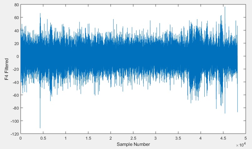
Having removed the anomalies from the signals, we can now use the fully conditioned signals in our analysis. Of course, the MATLAB code can be modified to remove other segments of the recorded signals should other sections also have distortions needing removal. If you do then remember to adjust the code to keep all of the signals and the time and sample counts equal to each other so that they are easier to line up with your script during your analysis.
Next steps
In my next section I analyze these conditioned signals in MATLAB. Check it out here. I also have made a fair number of EEG recordings available on the next page!